Differential Analysis - SysBio-Network Book

To investigate the role of TGF-β in kidney fibrosis, we will analyze and integrate transcriptomic, phosphoproteomic, proteomic, and secretomic data from kidney cells treated with TGF-β after 96 hours. We’ll begin by identifying genes, proteins, phosphorylation sites, and secreted proteins that show changes in response to TGF-β stimulation.

These differentially expressed features will later be used to infer the activity of regulatory proteins such as kinases and transcription factors, and to connect the various omics layers within a network context.

This tutorial starts from preprocessed, filtered, and normalized datasets for each modality and performs differential analysis using the limma package (Ritchie, 2015).

4.2.1.1Load Packages¶

import os
import pandas as pd
import numpy as np
import rpy2.robjects as ro
from rpy2.robjects import pandas2ri
from rpy2.robjects.packages import importr
import matplotlib.pyplot as plt
import seaborn as sns

We will use the R package limma for differential expression analysis. To make it accessible from this Python notebook, we’ll load it via the rpy2 interface.

# Activate pandas2ri for DataFrame conversion
pandas2ri.activate()

# Import R packages
limma = importr("limma")
base = importr("base")

4.2.1.2Load Data¶

All of the data needed to follow this tutorial are available in the SysBio Zenodo repository and will be downloaded within this script.

4.2.1.2.1Transcriptomics¶

The transcriptomics dataset contains normalized gene expression counts for each sample. These values typically come from RNA-seq data that has been normalized for sequencing depth and gene length.

# will be downloaded from Zenodo 
rna_file='../../data/multiomics_rna_data.csv' # will be downloaded from Zenodo 
rna_meta_file='../../data/multiomics_rna_meta.csv'

rna_matrix = pd.read_csv(rna_file, index_col=0) 
rna_metadata = pd.read_csv(rna_meta_file, index_col=0) 

# Prepare metadata and select comparison (TGF vs crtl)
rna_metadata["condition"] = pd.Categorical(rna_metadata["condition"], categories=["ctrl", "TGF"], ordered=True)

# Plot head of the count matrix
rna_matrix.head()

4.2.1.2.2Proteomics¶

The proteomics data includes normalized protein abundance measurements per sample obtained from mass spectrometry.

# will be downloaded from Zenodo 
prot_file='../../data/multiomics_proteomics_data.csv' # will be downloaded from Zenodo 
prot_meta_file='../../data/multiomics_proteomics_meta.csv'

prot_matrix = pd.read_csv(prot_file, index_col=0) 
prot_metadata = pd.read_csv(prot_meta_file, index_col=0) 

# Prepare metadata and select comparison (TGF vs crtl)
prot_metadata["condition"] = pd.Categorical(prot_metadata["condition"], categories=["ctrl", "TGF"], ordered=True)

# Plot head of the count matrix
prot_matrix.head()

4.2.1.2.3Phosphoproteomics¶

The phosphoproteomics dataset captures site-specific phosphorylation levels across samples.

# will be downloaded from Zenodo 
phospho_file='../../data/multiomics_phospho_data.csv' # will be downloaded from Zenodo 
phospho_meta_file='../../data/multiomics_phospho_meta.csv'

phospho_matrix = pd.read_csv(phospho_file, index_col=0) 
phospho_metadata = pd.read_csv(phospho_meta_file, index_col=0) 

# Prepare metadata and select comparison (TGF vs crtl)
phospho_metadata["condition"] = pd.Categorical(phospho_metadata["condition"], categories=["ctrl", "TGF"], ordered=True)

# Plot head of the count matrix
phospho_matrix.head()

4.2.1.2.4Secretomics¶

The secretomics data represents protein abundance in the secreted fraction of the samples. It reflects changes in the extracellular proteome in response to TGF-β treatment.

# will be downloaded from Zenodo 
secretomics_file='../../data/multiomics_secretomics_data.csv' # will be downloaded from Zenodo 
secretomics_meta_file='../../data/multiomics_secretomics_meta.csv'

secretomics_matrix = pd.read_csv(secretomics_file, index_col=0) 
secretomics_metadata = pd.read_csv(secretomics_meta_file, index_col=0) 

# Prepare metadata and select comparison (TGF vs crtl)
secretomics_metadata["condition"] = pd.Categorical(secretomics_metadata["condition"], categories=["ctrl", "TGF"], ordered=True)

# Plot head of the count matrix
secretomics_matrix.head()

4.2.1.3Differential Analysis¶

To perform differential analysis across all omics layers, we will first organize the datasets into a dictionary, where each entry corresponds to a specific modality. This structure allows us to loop through the modalities efficiently and apply the same differential analysis workflow to each one in a consistent and reproducible manner.

matrix_dict = {
    "transcriptomics": rna_matrix,
    "proteomics": prot_matrix,
    "phosphoproteomics": phospho_matrix,
    "secretomics": secretomics_matrix
    }

meta_dict = {
    "transcriptomics": rna_metadata,
    "proteomics": prot_metadata,
    "phosphoproteomics": phospho_metadata,
    "secretomics": secretomics_metadata
    }

limma_dict = {}

# Perform differential expression analysis for each omics type
for omics_type, matrix in matrix_dict.items():
    print(f"Performing differential analysis for {omics_type}...")

    # Convert pandas DataFrame to R DataFrame
    r_matrix = pandas2ri.py2rpy(matrix)
    r_metadata = pandas2ri.py2rpy(meta_dict[omics_type])

    # Assign the converted objects to R's global environment
    ro.globalenv["r_data"] = r_matrix
    ro.globalenv["r_meta"] = r_metadata
    ro.globalenv["omics"] = omics_type

    # Run Limma in R
    ro.r('''
    library(limma)

    # Convert Python data to R format
    count_matrix <- as.matrix(r_data)
    metadata <- r_meta

    # Design matrix for differential analysis
    if (omics != "secretomics"){
        design <- model.matrix(~ 0 + condition, data=metadata)
    } else {
        # For secretomics, include replicate in the design matrix
        design <- model.matrix(~ 0 + condition + replicate, data=metadata)
    }
    contrast <- makeContrasts(TGF_vs_ctrl = conditionTGF - conditionctrl, levels=design)

    # Fit Limma model
    fit <- lmFit(count_matrix, design)
    fit <- contrasts.fit(fit, contrast)
    fit <- eBayes(fit)

    # Extract differential expression results
    results <- topTable(fit, coef="TGF_vs_ctrl", number=Inf, adjust="BH")
    results$Feature <- rownames(results)
    results
    ''')

    # Convert R output back to Python DataFrame
    rna_de = pandas2ri.rpy2py(ro.r['results'])

    # Store results in the dictionary
    limma_dict[omics_type] = rna_de

Performing differential analysis for transcriptomics...
Performing differential analysis for proteomics...
Performing differential analysis for phosphoproteomics...
Performing differential analysis for secretomics...

We then visualise the results of the differential anaylsis in a volcano plot.

# Plot results
fig, axes = plt.subplots(1, 4, figsize=(12, 4))
axes = axes.flatten() 

for i, (name, df) in enumerate(limma_dict.items()):
    ax = axes[i]
    
    # Your custom plot code here, directing plots to the ax object
    # For example, a volcano plot:
    fc_thresh, p_thresh = np.log2(1.5), 0.05
    df['sig'] = np.where((df['adj.P.Val'] < p_thresh) & (df['logFC'] > fc_thresh), 'Up',
                np.where((df['adj.P.Val'] < p_thresh) & (df['logFC'] < -fc_thresh), 'Down', 'NS'))

    ax.scatter(df['logFC'], -np.log10(df['adj.P.Val']), 
                c=df['sig'].map({'Up': '#D62728', 'Down': '#1F77B4', 'NS': '#CCCCCC'}),
                alpha=0.6)
    ax.axhline(-np.log10(p_thresh), linestyle='--', color='black')
    ax.axvline(fc_thresh, linestyle='--', color='black')
    ax.axvline(-fc_thresh, linestyle='--', color='black')

    ax.set_title(name)
    ax.set_xlabel("log2 FC")
    ax.set_ylabel("-log10 adj.P")

plt.tight_layout()
plt.show()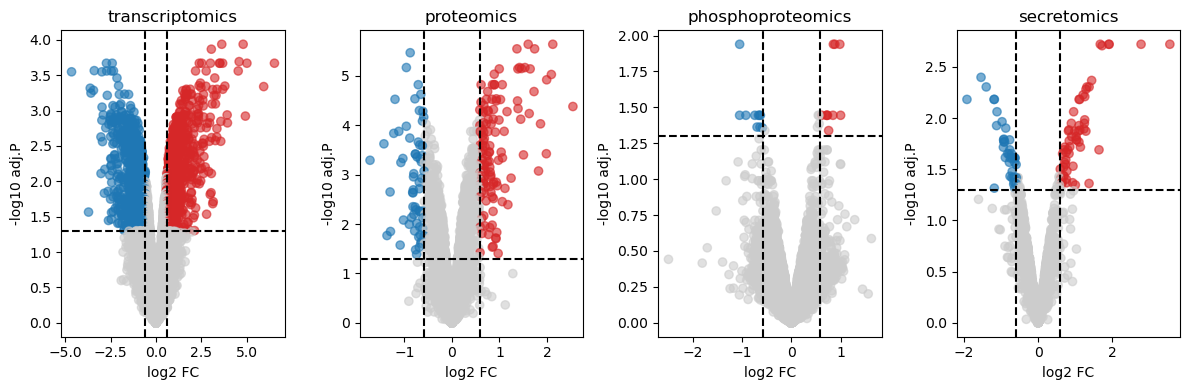

4.2.1.4Save Data¶

Finally, we will store the results of the differential analysis for each data modality. These results will serve as the input for our downstream analyses, including the inference of the activity of transcription factors and kinases, which we will perform in the next step of this workflow.

os.makedirs('results', exist_ok=True)

limma_dict['transcriptomics'].to_csv('results/rna_de.csv', index=False)
limma_dict['proteomics'].to_csv('results/proteomics_de.csv', index=False)
limma_dict['phosphoproteomics'].to_csv('results/phospho_de.csv', index=False)
limma_dict['secretomics'].to_csv('results/secretomics_de.csv', index=False)

References¶

Ritchie, M. E., Phipson, B., Wu, D., Hu, Y., Law, C. W., Shi, W., & Smyth, G. K. (2015). limma powers differential expression analyses for RNA-sequencing and microarray studies. Nucleic Acids Research, 43(7), e47–e47. 10.1093/nar/gkv007

SysBio Book

Multi-Omics Workflow