1.4Network contextualization with differential proteomics data

# version should be < 2 for pcst_fast compatibility
import numpy as np
print(np.__version__)

import gdown
import os

# File paths and their corresponding Google Drive IDs
files_to_download = {
    "op_signor.csv": "1Ooq4gUlpwZYvUOT3OEueJrqKQyZbxQly",
    "luad_de.csv": "1naFI56Wc2glkIn6CG4HJMGRwddxZacME"
}

# Download only if file doesn't exist
for filename, file_id in files_to_download.items():
    if not os.path.exists(filename):
        print(f"⬇️  Downloading {filename}...")
        gdown.download(id=file_id, output=filename)
    else:
        print(f"✅ {filename} already exists. Skipping download.")

import seaborn as sns
import matplotlib.pyplot as plt
import pandas as pd
import numpy as np

from pcst_fast import pcst_fast
import networkx as nx

signor = pd.read_csv('op_signor.csv')
signor = nx.from_pandas_edgelist(signor[['source_genesymbol', 'target_genesymbol']].rename(columns={'source_genesymbol': 'source', 'target_genesymbol': 'target'}))
signor.number_of_edges(), signor.number_of_nodes()

luad = pd.read_csv('luad_de.csv')
luad['significance'] = -np.log10(luad['adj.P.Val'])
sns.scatterplot(data = luad, x = 'logFC', y ='significance')

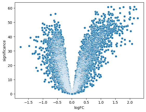
luad.sort_values(by='significance', ascending=False, inplace=True)
luad.head(10)

# subset graph to nodes in the luad
signor_luad = signor.subgraph(luad['protein']).copy()
abs_fc_dict = dict(zip(luad['protein'], np.abs(luad['logFC'])))
nx.set_node_attributes(signor_luad, abs_fc_dict, 'logFC')
signor_luad.number_of_edges(), signor_luad.number_of_nodes()

def solve_pcst(
        G: nx.Graph,
        prize_attr: str = "logFC",
        edge_cost: float = 1.0,
        pruning: str = "strong",
        verbosity: int = 0,
        num_clusters: int = 1
    ) -> nx.Graph:
        """
        Solves a PCST using node prizes and a fixed edge cost (regularization).

        Args:
            G (nx.Graph): Graph with node attribute `prize_attr`.
            prize_attr (str): Node attribute key to use as prize value.
            edge_cost (float): Constant edge cost for all edges.
            pruning (str): Pruning strategy ('none', 'simple', 'gw', or 'strong').
            verbosity (int): Verbosity level (0 for silent, 1 for verbose).
            num_clusters (int): Number of desired output components.

        Returns:
            nx.Graph: Subgraph induced by the PCST solution.
        """
        node_list = list(G.nodes())
        node_to_idx = {node: i for i, node in enumerate(node_list)}
        idx_to_node = {i: node for node, i in node_to_idx.items()}

        edge_list = []
        cost_list = []
        edge_lookup = []

        for u, v in G.edges():
            edge_list.append([node_to_idx[u], node_to_idx[v]])
            cost_list.append(edge_cost)
            edge_lookup.append((u, v))

        edge_array = np.array(edge_list, dtype=np.int64)
        cost_array = np.full(len(edge_list), edge_cost, dtype=np.float64)

        prizes = np.array([
            G.nodes[node].get(prize_attr, 0.0) for node in node_list
        ], dtype=np.float64)

        prizes = np.abs(prizes)

        root_idx = -1

        selected_nodes_idx, selected_edges_idx = pcst_fast(
            edge_array, prizes, cost_array, root_idx, num_clusters, pruning, verbosity
        )

        selected_nodes = {idx_to_node[i] for i in selected_nodes_idx}
        selected_edges = []
        for edge_idx in selected_edges_idx:
            u, v = edge_lookup[edge_idx]
            if u in selected_nodes and v in selected_nodes:
                selected_edges.append((u, v))

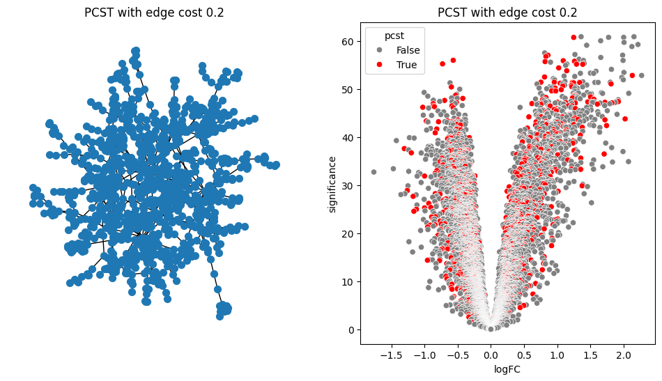
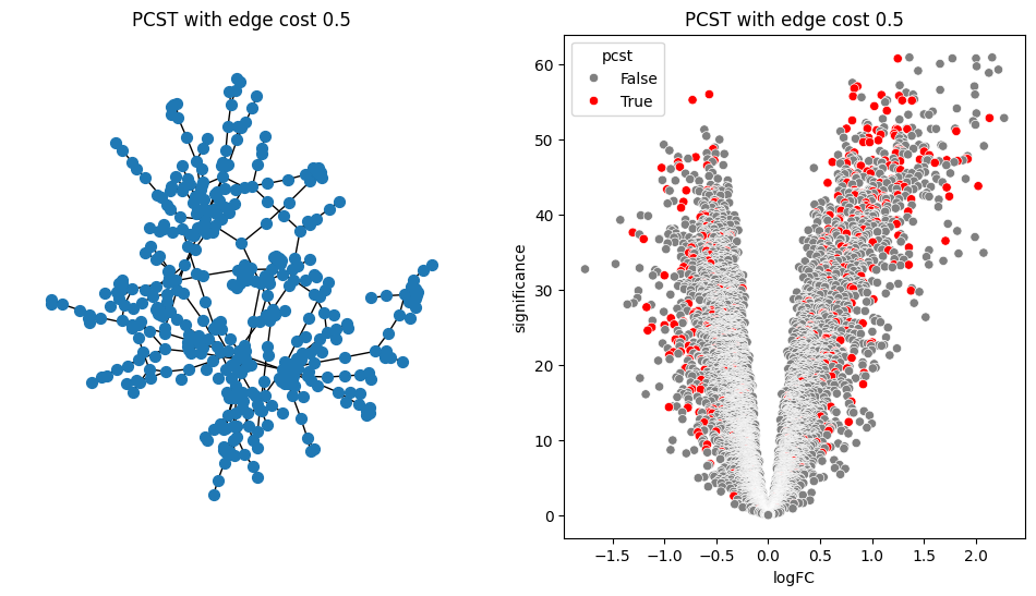
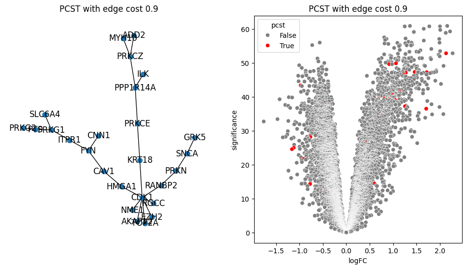
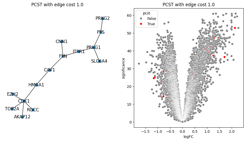
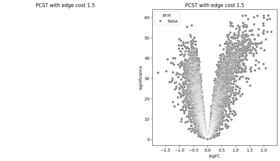
        return G.edge_subgraph(selected_edges).copy()

for i in [0.2, 0.5, 0.9, 1.0, 1.5]:
    pcst = solve_pcst(signor_luad, edge_cost=i)
    fig, axs = plt.subplots(1, 2, figsize=(12, 6))
    pos = nx.spring_layout(pcst)
    lab = len(pcst.nodes()) <= 100
    nx.draw(pcst, pos, with_labels=lab, node_size=50, ax=axs[0])
    luad['pcst'] = luad['protein'].isin(pcst.nodes())
    sns.scatterplot(data=luad, x='logFC', y='significance', hue='pcst', palette=['gray', 'red'], ax=axs[1])
    axs[0].set_title(f'PCST with edge cost {i}')
    axs[1].set_title(f'PCST with edge cost {i}')

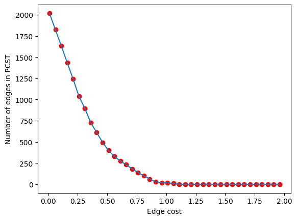
lambdas = np.arange(0.01, 2, 0.05)
pcst_size = []
for i in lambdas:
    pcst = solve_pcst(signor_luad, edge_cost=i)
    pcst_size.append(len(pcst.edges()))

plt.plot(lambdas, pcst_size)
plt.xlabel('Edge cost')
plt.ylabel('Number of edges in PCST')
plt.scatter(lambdas, pcst_size, color='red')